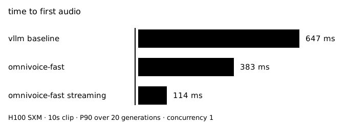
State of the art text-to-speech (TTS) models fall into two buckets today.
Autoregressive (AR): as the name suggests, these generate one audio token at a time and can therefore be streamed. Qwen3-TTS and Voxtral-4B-TTS-2603 are good examples. These typically keep their time to first audio (TTFA) within 250 ms, and are widely used in latency-sensitive applications like voice agents.
Non-autoregressive (NAR): these models iteratively denoise the audio tokens through diffusion or its adjacent technique, flow matching. Because they generate all tokens at once, their time to first audio equals the time to generate the full audio; at least by default. OmniVoice and F5-TTS are popular examples. Their latency depends on the generated audio length, at least 600 ms for 10 seconds of audio.
A couple reasons to care about NAR and its latency. a.) NAR models empirically excel at sounding humanlike when cloning a voice. b.) Voice agents are a big use case for TTS, and there’s a tight latency target for the STT → LLM → TTS cascade. Getting NAR latency on par with AR opens it up for voice agents.
Here’s how it sounds.
In this series of posts, we’ll start with OmniVoice’s vLLM-Omni baseline and iteratively optimize it.
- Part 1: Understand how the model works; run baselines and find the bottlenecks. (this post)
- Part 2: Beat the vLLM baselines and get OmniVoice to sub-120 ms with blockwise streaming.
- Part 3: This is an auto-research-shaped systems problem with clean verifiability. We’ll run Codex and Claude Code in parallel and see how much each can recover.
If you just want the model with the lowest advertised streaming latency of 120 ms, with all the optimizations from Parts 1 and 2 baked in, use omnivoice-fast.
Audio Tokenization
The first step is understanding how the model represents audio. Similar to how a text tokenizer converts text into a series of numbers, an audio tokenizer converts an audio file into a list of discrete numbers.
Let’s get concrete. The OmniVoice model uses the Higgs Audio v2 tokenizer, so let’s see how it represents 10 seconds of audio.
Assume you have an audio.wav file on disk, 10 seconds long at 24 kHz (a good default). That means each second of audio has 24,000 samples of sound data. Think of each one as the pressure on the speaker at a point in time, ranging from -1 to 1 after normalization. This is how we represent a continuous sound wave: by sampling it 24k times per second.
The goal of a tokenizer is to encode this into fewer datapoints and reconstruct it back as accurately as possible, i.e. decoder(encoder(audio)) ~ audio.
The Higgs v2 tokenizer operates at 25 fps, so each frame spans 1000/25 = 40 ms. The encoder takes each 40 ms frame and returns 8 numbers, [c0, c1, c2 .. c7], where each can range from 0 to 1023. So 40 ms of sound is represented by 8 numbers, one from each codebook. You can think of it like binary, where the most significant bit carries the most value and the rest iteratively refine and shape the audio.
Mental map, for most audio, reconstruction using 4-6 codebooks sounds fine vs 8.
Here’s a visualisation. You can see that the first 4 codebooks already give you a good enough outline.
To appreciate the tokenizer, let’s look at the information density:
- A 40 ms frame of 24 kHz audio is
40 * 24 * 16 bits = 15360 bits - That same 40 ms after encoding is
8 codebooks * 10 bits = 80 bits. 192x reduction
You can think of a 40 ms frame as the atomic unit the model operates on and it's represented by 8 numbers.
OmniVoice Architecture
To understand how the model works, let’s think in inputs and outputs, and how we can transform one into the other.
input  -> [target_text]
output -> [target_audio]
Shapes:
target_text→ "Hello, this is a target text" → tokenize →[9707, 11, 419, 374, 264, 2169, 1467]tokens. Each number can be from 0 to 150k.T_textis the number of text tokens, which is 7 here.target_audio→ let's say it's 5s → 5 × 25 = 125 output frames using the Higgs tokenizer → tensor of shape[8 × 125]. Each number can be from 0 to 1023. 125 is the time axis.
![A 5-second 24 kHz waveform is encoded by the Higgs v2 tokenizer at 25 fps into a [8 × 125] grid of int10 tokens. Each row is one of 8 codebooks; each column is a 40 ms frame; each cell is an integer between 0 and 1023.](figures/audio-shape.svg)
We do have some hints. The abstract of the paper says it’s a NAR (non-autoregressive) diffusion model with a bidirectional LLM backbone. Diffusion means you start with a noisy grid and iteratively denoise some cells after each forward pass, and the [8 × 125] codebook × time grid seems a perfect candidate for that noisy grid.
A reasonable first assumption: you pass [T_text, model_dim] through the model, it gets enriched semantically layer by layer, and at the end you have a [T_text, model_dim] tensor. Now we need a way to turn [T_text, model_dim] into [8 × 125].
Two things:
- A way to expand the text-length dimension into the audio-length dimension (
T_text -> 125). - A way to convert the model’s internal space (text) into audio/codebook space.
This is a valid (old) way of doing things, and the paper’s abstract rules it out:
“Unlike conventional discrete NAR models that suffer from performance bottlenecks in complex twostage (text-to-semantic-to-acoustic) pipelines, OmniVoice directly maps text to multi-codebook acoustic tokens”
So after a forward pass, the model directly predicts audio tokens. It does this in a clever way: instead of using only text tokens as input, we add audio tokens to the input as well.
But we don’t know the audio tokens yet, predicting them is the whole goal. So at the start we mark them with a special mask token, signifying they’re still unknown.
Concretely, given the input “Hello, this is a target text”: along with [T_text, model_dim], we allot some tokens for the audio. We assume the text will be 5s, so we allot 125 audio tokens. The input is then [T_text + T_audio, model_dim], where T_text = 7 and T_audio = 125.
| variable | what it is | here |
|---|---|---|
target_text | the input text string | "Hello, this is a target text" |
T_text | number of text tokens | 7 |
target_audio | the output audio tokens (codebook × time grid) | [8 × 125] |
T_audio | number of audio frames (the time axis) | 125 |
model_dim | the model's internal embedding width | 1024 |
target_text -> [T_text, model_dim] is simple: embed(tokenize(target_text)).
target_audio_masked -> [T_audio, model_dim] is slightly more involved. We have separate audio embeddings for each of the 8 codebooks and do a weighted sum to get a single embedding per frame.
Similarly, after the forward pass, we have audio heads (essentially unembeddings) to convert [T_audio, model_dim] back into [8, T_audio, 1025].
We finally got the output shapes right.
Iterative Demasking
The only remaining part is the masked tokens: how are we unmasking them? After each forward pass we need to unmask/commit at least one of the tokens in the [8 × 125] grid we talked about, replacing the mask token with an actual value from 0 to 1023 for a codebook.
Otherwise the inputs won’t change between steps. The only way information propagates is by unmasking some audio tokens and changing their input embeddings.
Say we have 32 steps and 125 * 8 token positions to unmask, and each step should unmask at least one position. At each step we need to figure out:
- How many positions to unmask.
- Which of them to unmask.
- The unmasking strategy: how we pick a token for a position.
OmniVoice uses this inference strategy:
- A heavily back-loaded schedule. Step 1 commits just 3 tokens out of 1000. After 16 of 32 steps, only ~9% are committed.
- Position selection. Confidence per position is the max log-prob. Earlier codebooks get a layer-penalty boost so they commit before later ones. We sample x positions weighted by these.
- Token assignment. Once the positions are decided, for each one we just pick the token with the highest confidence value, i.e. argmax.
Tbh it feels pretty adhoc and quite different from how they train. But a side benefit is that there are so many knobs you can tweak to speed up inference.
Interactive visualization of OmniVoice's 32-step iterative demasking on an 8-codebook by 40-frame grid. Drag the slider or press play to step through. Lower codebooks tend to commit first, and most tokens commit in the final steps.
Model and Hardware Setup
Now let’s define the model config and hardware numbers we’ll use for the roofline calculations.
Model config
| parameter | value |
|---|---|
num_steps | 32 |
| transformer | Qwen3 0.6B |
| audio tokenizer | Higgs v2 |
n_dim | 1024 |
n_layers | 28 |
n_attention_heads | 8 |
llm_text_vocab_size | 151,676 |
| precision | bfloat16 |
num_steps = 32 means the model runs 32 forward passes through the bidirectional transformer. Each forward pass goes through 28 transformer layers.
GPU numbers
H100 SXM:
| quantity | value |
|---|---|
| BF16 sparse | 1,979 TFLOP/s |
| BF16 dense | 989 TFLOP/s |
| memory bandwidth | 3.35 TB/s |
For simplicity, I’ll use:
compute = 1e15 FLOP/s
memory  = 3e12 bytes/s
Here’s a rough pseudocode that’s representative of the main calculations in the model.
tokenize(input_text)

for i in range(32):
    embed_audio()
    transformer()
    audio_head()  # de embed audio
    sample()      # unmask some positions

decode()
Baseline Latency Breakdown
Here’s a text that generates exactly 10s of audio:
“Gollum leads Frodo and Sam to the well-defended Black Gate, and recommends another route to them. Frodo and Sam are captured by Faramir’s Rangers.”
The text is 36 tokens, and 10s of audio is 25 * 10 = 250 tokens - so 286 overall, which we’ll round to 300 for our calculations. The batch size is 2 because of classifier-free guidance; each forward pass runs once conditioned on the text and once unconditioned, then combines the logits. 300 × 2 = 600 tokens per forward pass.
0 ──────────────────────────────────────────────────────────── 784 ms
    │
    ├── 32 × embed                     1.4 ms
    ├── 32 × 28 transformer layers   740.2 ms
    │   ├── attention work           415.1 ms
    │   ├── MLP work                 280.2 ms
    │   └── norms (in + post)         44.9 ms
    ├── 32 × audio_head                8.9 ms
    ├── 32 × sampling                 23.6 ms
    └──  1 × decoder (DAC stack)       9.7 ms
We got our baseline. As expected, you immediately notice the transformer backbone is taking the bulk of the time. You might notice that the chart at top says 647 ms and we measure 784 ms here. It’s from profiling overhead. The later numbers stay apples-to-apples with this 784 ms.
Roofline Analysis
A roofline is a quick way to ask: given the hardware above, is this model/operation limited by compute, memory bandwidth, or something else? As we’ll see, a large gap between theoretical and measured times means something’s wrong. The Scaling Book has a great chapter on this.
Audio Head
To get a feel for running theoretical rooflines for compute and memory, we’ll start with the audio head, which is comparatively simple. Empirically, it takes 8.9 ms.
To recap, the audio head runs after the transformer. It essentially converts the [T, n_dim] hidden states into [8, T, 1024], an unembedding from model space into codebook/audio space.
Here’s the exact code from the vLLM implementation:
# Prediction head: hidden → 8 * 1025
self.audio_heads = nn.Linear(
    config.llm_hidden_size,
    config.num_audio_codebook * config.audio_vocab_size,
    bias=False,
)

def _get_logits(self, hidden_states: torch.Tensor) -> torch.Tensor:
    """Project hidden states to per-codebook logits.

    Args:
        hidden_states: [B, S, hidden_size]

    Returns:
        logits: [B, 8, S, 1025]
    """
    batch_size, seq_len, _ = hidden_states.shape
    logits_flat = self.audio_heads(hidden_states)  # [B, S, 8*1025]
    return logits_flat.view(
        batch_size,
        seq_len,
        self.config.num_audio_codebook,
        self.config.audio_vocab_size,
    ).permute(0, 2, 1, 3)  # [B, 8, S, 1025]
We noted earlier that llm_hidden_size is 1024 and audio_vocab_size is 1025, with 8 codebooks, so the weight is a [1024, 8*1025] matrix.
Compute. With T = 600, we multiply [600, 1024] by [1024, 8200]. That’s 600 * 1024 * 8200 * 2 floating point operations, where one floating point operation is a single add or multiply. (It’s a good exercise to work out where the 2 comes from.) That comes out to 10,076,160,000, or about 1e10.
An H100 gives us 1e15 FLOP/s, so each step costs 1e10 / 1e15 = 10 µs. Over 32 steps, that’s 0.32 ms.
Memory. The computation needs three accesses:
- Load activations:
[600, 1024]× 2 bytes (BF16) = 1.2 MB - Load audio-head weights:
[1024, 8200]× 2 = 16.8 MB - Write activations back:
[8, 600, 1025]× 2 = 9.8 MB
That’s 28 MB. At 3e12 bytes/s, the time is 28e6 / 3e12 = 9 µs per step, or 0.3 ms over 32 steps.
Here’s a more formal version if you’d prefer it. We’ll use this format for later sections:
Audio head - one step:
  Compute
    C   = 600 × 1024 × 8200 × 2  ≈ 1.0e10 FLOP
    t_c = C / P = 1.0e10 / 1e15  ≈ 10 µs

  Memory                          bytes
    load  activations  600×1024×2   1.2 MB
    load  weights     1024×8200×2    17 MB
    store output    8×600×1025×2    9.8 MB
    M   = Σ                          28 MB
    t_m = M / B = 28 MB / 3 (TB/s)  ≈ 9 µs

  Roofline
    t   = max(t_c, t_m) = max(10, 9) ≈ 10 µs / step
        × 32 steps                   ≈ 0.32 ms
Compute and memory usually overlap rather than waiting on each other, so Time = max(compute_time, memory_time). Here that’s 0.32 ms. It’s pretty interesting that the two come out so close.
Precision Mismatch
But if you look at the measured time, it’s 8.9 ms. It’s 27x higher than theoretical. Something’s off! This is exactly why rooflines are valuable. We don’t know exactly what’s wrong yet, but it gave us a strong enough reason to go take a look.
We wanna measure how much time each kernel is taking. For faster iteration, we run this on a standalone audio head with the same shapes.
| kernel | % time |
|---|---|
sm80_xmma_gemm_f32f32_f32f32_f32_tn_n_tilesize64x64x8_stage3_warpsize… |
100.00% |
We see that there’s only 1 kernel, running matmul as expected. Notice anything interesting?
It’s running FP32 and not BF16 like we were calculating theoretically. An H100 has max 67 FP32 TFLOP/s vs ~1000 for BF16.
But why is the model running at full precision? Qwen3 0.6B supports BF16 by default and the paper clearly mentions training in mixed precision.
“Mixed precision (BF16) and sequence packing (8192 tokens per GPU) are employed during training to improve efficiency.”
BF16 Results
Let’s move the standalone audio head to BF16 and run again.
| per call | × 32 calls | |
|---|---|---|
| theoretical BF16 roofline | 9.5 µs | 0.32 ms |
| observed FP32 production | 273.04 µs | 8.9 ms |
| observed BF16 production | 32.98 µs | 1.06 ms |
A big win! It decreased 8x.
And to be clear about what this means: this is vLLM-Omni - the reference serving engine - silently running in full precision as the default. And it’s not just the audio head: you’ll see below that the MLP drops from 280 ms to 73 ms under BF16 too, which means the whole transformer was running FP32.
You might notice that there’s still a 3x gap from theoretical rooflines. It’s from a third bound called launch overhead, which comes from the CPU. We’ll discuss this in detail in later sections.
MLP
Let’s get whole-model baselines again after moving to BF16. We’ll keep the norms, sampling and decoder in FP32, as they’re relatively low compute and generally require high precision.
0 ───────────────────────────────────────────────────── 696 ms
    │
    ├── 32 × embed                     4.3 ms
    ├── 32 × 28 transformer layers   599.9 ms
    │   ├── attention work           399.3 ms
    │   ├── MLP work                  73.7 ms
    │   └── norms (in + post)        126.9 ms
    ├── 32 × audio_head                1.5 ms
    ├── 32 × sampling                 77.5 ms
    └──  1 × decoder (FP32)           12.5 ms
Not a great win, as we expected. MLP reduced big from 280 to 73, but norms and sampling increased because we’re doing a bunch of .to(cast) operations from BF16 to FP32, which is killing the gains.
MLP        280→ 74  ██████████████████│          −206
attention  415→399                  ▍█│           −16
audio_head   9→  2                   ▋│            −7
embed        1→  4                    │▎           +3
decoder     10→ 12                    │▎           +3
sampling    24→ 78                    │████▊      +54
norms       45→127                    │███████▏   +82
                              ▋███████│
net: −88 ms. most of the MLP win lost to cast overhead
As an exercise, let’s calculate the rooflines for MLP and double-check whether we’re leaving any performance on the table.
You might ask: attention is clearly the bottleneck, so why are we looking at MLP? But as we noticed before, a bottleneck slowing one component usually touches other parts of the model too. MLP is a simpler operation than attention and should be easier to roofline. It’s literally 5 lines.
class OmniVoiceMLP(nn.Module):
    """Qwen3-style MLP with SwiGLU."""

    def __init__(self, config: OmniVoiceConfig):
        super().__init__()
        self.gate_proj = nn.Linear(config.llm_hidden_size, config.llm_intermediate_size, bias=False)
        self.up_proj   = nn.Linear(config.llm_hidden_size, config.llm_intermediate_size, bias=False)
        self.down_proj = nn.Linear(config.llm_intermediate_size, config.llm_hidden_size, bias=False)

    def forward(self, x: torch.Tensor) -> torch.Tensor:
        return self.down_proj(F.silu(self.gate_proj(x)) * self.up_proj(x))
Here are the shapes of the matrices:
up_proj -> [1024, 3072]gate_proj -> [1024, 3072]down_proj -> [3072, 1024]
We’ll treat the SiLU non-linearity as negligible.
MLP - one layer
shapes:  up,gate [1024 → 3072]   down [3072 → 1024]

  Compute                          (3 matmuls)
    each  600 × 1024 × 3072 × 2   ≈ 3.8e9 FLOP
    C   = 3 × 3.8e9               ≈ 11 GFLOP
    t_c = C / P = 11e9 / 1e15     ≈ 11 µs

  Memory                           bytes
    load  weights  3×(1024×3072×2)   19 MB
    load  act in       600×1024×2   1.2 MB
    store up,gate,silu 3×(600×3072×2) 11 MB
    store down out     600×1024×2   1.2 MB
    M   = Σ                          32 MB
    t_m = M / B = 32 MB / 3 (TB/s)  ≈ 11 µs

  Roofline
    t   = max(t_c, t_m) = max(11, 11) ≈ 11 µs / layer
        × 32 steps × 28 layers        ≈ 10 ms
Surprisingly, it’s very close again.
total time = 11 µs * 32 * 28 layers = 10 ms
But we’re seeing 73 ms, so there’s still a lot of juice left. Let’s look at the bottleneck.
Recap: What We Learned
- Diffusion TTS is slow because, for TTFA, we do a full transformer forward pass 32 times, vs Autoregressive TTS generating one token at a time through a single forward pass.
- The baseline was 784 ms for vLLM-Omni for generating 10 seconds of audio.
- We started with the simple audio head to build intuition for writing rooflines. The audio head, which should’ve taken ~0.32 ms, was measuring 8.9 ms. A 27x gap.
- We looked at its kernels and found that 100% of its time was spent in an FP32 kernel, and that the entire model was also running on FP32 by default, when both the OmniVoice TTS and its Qwen3 transformer backbone support BF16.
- Takeaway: running the rooflines revealed that something was wrong, which made us take a deeper look and find the precision mismatch.
What’s Next
We’ve seen that MLP responded very well to BF16 (4x drop), but attention barely moved. It’s 57% of total runtime (≈400 ms even after BF16), and we haven’t roofline’d it yet. In a typical transformer, MLP/attention compute is 2:1. MLP was compute-bound, so fixing the precision helped a lot, while attention is bound by something else (maybe memory or launch overhead).
Answer: yes, it’s launch overhead. We’ll tackle that and build blockwise streaming to get to 120 ms in the next part.
Acknowledgements
Thanks to Prasad Kawthekar, Krish Sharma and Michael McCanna for providing valuable feedback on earlier drafts of this post.